
Using pre-calculated H3 cells with Icon Map
Icon Map is capable of taking longitude and latitude coordinates and automatically generating an H3 hexagon cell at the required resolution to render on the map. It's a great way of aggregating lots of point data to show trends and patterns that still allows you to interact with those values to show the makeup of the underlying rows of data.
Icon Map generates H3 cells from longitude and latitude coordinates
The report below contains crime data in London - you can click on one of the H3 cells and it will show the breakdown of crime and show the individual locations on the smaller map.
In this example we pass into Icon Map a unique location ID, the longitude, the latitude and the sum of the number of crimes in each location.
Why pre-calculate H3 cell IDs?
So if Icon Map can aggregate the data for us, why might we want to pre-process the data and send the aggregated values to the map?
Well the main reason is likely to be performance. In the example above we have around 40,000 locations that we're aggregating. This is a lot of data for a Power BI visual to be processing on the fly - in fact more than any of the 'out of the box' map visuals can deal with.
In the identical looking report below, we have the same H3 map, but this time instead of sending 40,000 rows of data to the map, we are only sending 364 - one row representing each H3 cell. We are also now only sending 2 columns (H3 cell ID, and the sum of the number of crimes) - a significant reduction in the size of the data sent as well as the number of rows.
Performance
The other benefit is that when we click on a cell on the map to cross-filter the other visuals, rather than Power BI filtering on hundreds or thousands of IDs, it only needs to filter on one. Much faster - and will work well with both Icon Map Pro and Slicer without needing Slicer's use of Power BI's filter API.
Suppression of sensitive data
Another reason we may need to pre-process the data to generate the H3 cells is data sensitivity. A customer contacted recently with the requirement to not display cells with fewer than 5 source locations. If we pre-process the H3 cells, we can filter out all cells with fewer than 5 original locations as part of the data-ingestion process. We then not only don't show these on the map, but we don't store them in the Power BI data model either, which is a much better solution from a security standpoint.
Source already provides H3 cell IDs
Another reason to use pre-calculated H3 cells IDs is that the source data you're working with already has the H3 cell IDs included. We see an increasing number of datasets being published using H3 cell IDs.
Calculating H3 Cell IDs with Power BI or Microsoft Fabric
So if we do want to calculate the cell IDs - what are our options? Power BI doesn't have geo-spatial data processing capability built in to the product, but there are plenty of options we can use.
Python Data Source in Power Query
Probably the easiest route to calculating H3 cell IDs is to use the Python data source in Power Query.
Let's walk through step by step how to configure this.
- If you don't already have Python installed, then download and install it from python.org.
- During the installation tick the 'Add python.exe to PATH' option
- After installation, run the following from the command prompt:
python -m pip install pandas matplotlib h3
This will install the pandas and matplotlib libraries that Power BI needs, plus the H3 library we will use to calculate our H3 cell IDs.
Now we have our Python setup ready, we can head to Power BI Desktop to ingest our data.
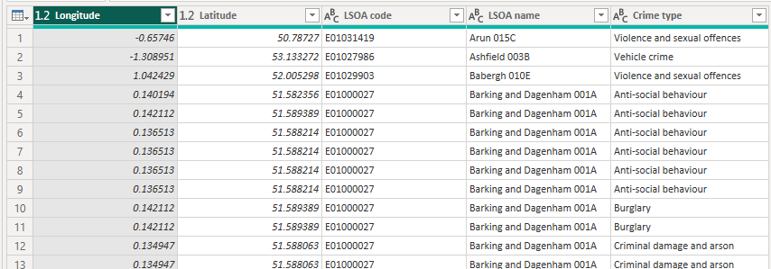
For simplicity, I'm just using a CSV source file downloaded from data.police.uk as my source data. I've used the CSV source in Power Query and then the UI to remove columns I'm not interested in resulting in the following data configuration:
We are now ready to execute our Python code to generate the H3 cell IDs. In the Transform tab, click the 'Run Python Script' button and paste the following code.
import h3
dataset['H3_Res7'] = dataset.apply(
    lambda r: h3.latlng_to_cell(r['Latitude'], r['Longitude'], 7),
    axis=1
)
Indentation is important in Python as it controls the flow of the code, so be careful when copying code.
You should now see the following:
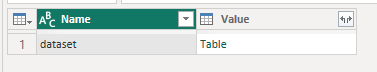
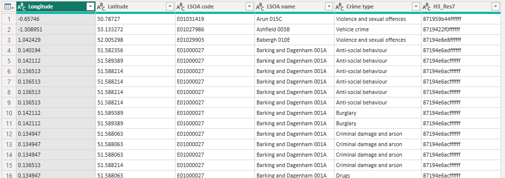
Click on the "Table" entry and you should now have a an additional column H3_Res7 with the H3 cell hex ID for each location.
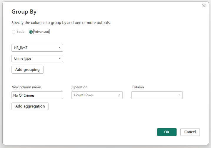
You can now remove the longitude and latitude data from your report if required, and if the data at a granular level is sensitive, you can use the Group By option in Power Query to group by the H3_Res7 field. For example:
You can then configure Icon Map's data mapping as follows:
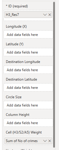
with the H3 cell ID field in the Location ID field, and the measure in the Cell Weight / H3 Weight field.
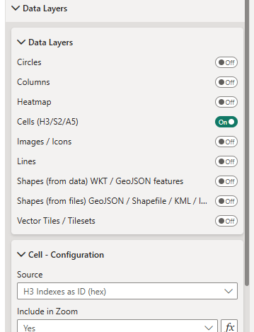
Then in the data layer formatting settings, enable the Cells / H3 data layer and select 'H3 Indexes as ID (hex)' as the source:
You can download the .pbix and source CSV files to see how this is constructed.
Other options for generating H3 cell IDs
Microsoft Fabric notebooks
If your data is already landing in Microsoft Fabric, a notebook can be a better place to calculate H3 cell IDs than Power Query. This keeps the geospatial preparation close to the lakehouse data and means the resulting table can be reused by Power BI reports, semantic models, pipelines and other Fabric items.
For interactive exploration, you can install the Python H3 library at the start of a notebook:
%pip install h3
Then calculate the H3 cell ID from latitude and longitude:
import h3
import pandas as pd

df = spark.read.table("street_crime").toPandas()

df["H3_Res7"] = df.apply(
    lambda r: h3.latlng_to_cell(r["Latitude"], r["Longitude"], 7),
    axis=1
)

spark.createDataFrame(df).write.mode("overwrite").saveAsTable("street_crime_h3")
For larger datasets, avoid converting everything to pandas. Use a Spark UDF instead:
import h3
from pyspark.sql.functions import udf, col
from pyspark.sql.types import StringType

@udf(StringType())
def latlng_to_h3(lat, lon):
    if lat is None or lon is None:
        return None
    return h3.latlng_to_cell(lat, lon, 7)

df = spark.read.table("street_crime")

df_h3 = df.withColumn(
    "H3_Res7",
    latlng_to_h3(col("Latitude"), col("Longitude"))
)

df_h3.write.mode("overwrite").saveAsTable("street_crime_h3")
Once the H3 index has been created, you can aggregate the data before it reaches Power BI:
from pyspark.sql.functions import count

df_grouped = (
    df_h3
    .groupBy("H3_Res7")
    .agg(count("*").alias("CrimeCount"))
    .filter(col("CrimeCount") >= 5)
)

df_grouped.write.mode("overwrite").saveAsTable("street_crime_h3_grouped")
This gives you a compact table containing one row per H3 cell. It is a good fit for Icon Map because the report only needs the H3 cell ID and the measure you want to visualize, rather than every original latitude and longitude.
For production or scheduled notebooks, consider using a Fabric Environment rather than relying on inline %pip install commands. This makes the notebook more repeatable and ensures package versions remain consistent across executions.
DuckDB in Fabric notebooks
DuckDB is another useful option inside a Fabric notebook, especially for smaller to medium-sized analytical preparation steps. Its H3 extension can create H3 cell IDs directly in SQL:
INSTALL h3 FROM community;
LOAD h3;

SELECT
    h3_latlng_to_cell_string(latitude, longitude, 7) AS H3_Res7,
    COUNT(*) AS CrimeCount
FROM street_crime
GROUP BY H3_Res7;
The important detail here is the coordinate order. DuckDB's H3 function uses latitude first, then longitude.
KQL in Fabric Real-Time Intelligence
If your data is in a Fabric Eventhouse or KQL database, you can calculate H3 cells directly with KQL:
StreetCrime
| extend H3_Res7 = geo_point_to_h3cell(Longitude, Latitude, 7)
| summarize CrimeCount = count() by H3_Res7
| where CrimeCount >= 5
This is particularly useful for streaming, telemetry or operational datasets where the data is already being queried in Real-Time Intelligence. The output can then be exposed to Power BI, with Icon Map configured to use the H3 cell ID as the location identifier.
KQL also supports converting an H3 cell back to its center point if you need a representative coordinate:
StreetCrimeH3
| extend Centre = geo_h3cell_to_central_point(H3_Res7)
As with the notebook approach, pre-calculating and aggregating the H3 cells before they reach the report can improve performance, reduce model size and help avoid exposing sensitive point-level locations.